Author: Rahul Goel (NetID: rg764)
I. Objective
The primary objective of this lab is to build a virtual map of a static room. The robot will be placed in five (5) marked locations around the room and spin around its axis while measuring the ToF readings. This will enable the robot to provide distance and degree information that can be utilized to create the map. Angular speed control (PD) was done on the raw gyroscope values and the readings from different positions were merged to form the map.
II. Materials/Software
- 1x Fully assembled robot with Artemis, ToF sensors, and an IMU sensor
- 1x USB A to C Cable
- 2x Li-ion 3.7V 650mAh (or more) Battery
III. Procedure/Design/Results
Lab Tasks Overview
The following tasks shall be accomplished as a part of this lab:
- Implement a PID/PD controller
- Transmit the distance, timestamp, and gyroscope values via BLE
- Collect the distance, timestamp, and gyroscope values on the computer
- Gather readings in the four/five locations in the room
- Sanity check the individuals turns by plotting them in polar and cartesian (rectangular) plot
- Merge plots
- Convert to Line-Based Map
PID/PD Controller – Angular Speed Control
Continuing from Lab 6, a PD controller is utilized which outputs the PWM duty cycle that is used to drive the motors. For more information on the PD controller, please refer to the Lab 6 write up. As seen in the code snippet below, the setpoint value (25) is subtracted from the rotational_speed value (readings from the gyroscope), and the subtracted value is fed into the PID_pass (PID controller computation), which then determines the PWM of the motors to rotate the robot about its axis. It was noticed that the most effective KP and KD values for slow and smooth turns was 4.5 and 1.5 respectively.
setSpeed(PID_pass(time_current, time_previous, error_previous, (rotational_speed - setPoint), I_sum));

float PID_pass(float time_current, float time_previous, float error_previous, float current_error, float I_sum)
{
 return (P*current_error) + (I*I_sum) + ((D*(current_error - error_previous))/(time_current - time_previous));
}
One of the methods used to perform smooth rotations was adding tape to the wheels. This decreased the friction and the jerking of the robot, in turn improving the quality of the sensor readings. However, the robot did turn a lot faster at first when the tape was put on, so the maximum PWM of the robot had to be decreased by about 30%.
Read Out Distances
Once the PID control is verified, the robot is ready to read out the distances. The robot is placed in five known locations in the room and turned around its axis to capture distance and degrees (degrees/second) information which will be used to create the virtual map. The robot is started in the same direction for all scans. While the robot slightly shifts from its starting point, it is believed that the shift not significant enough to cause great error.
Merge and Plot Readings
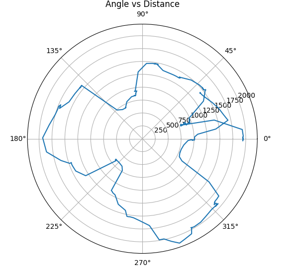
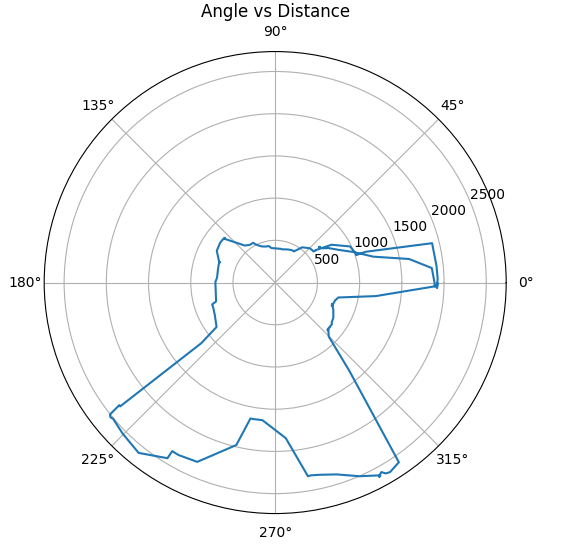
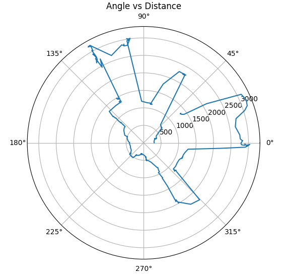
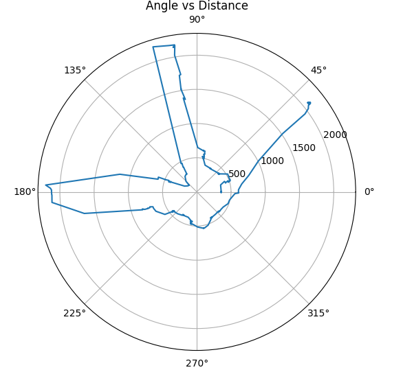
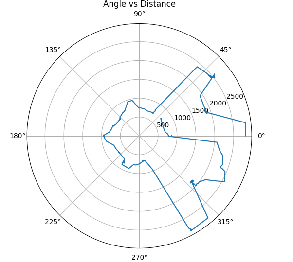
Five polar plots are formed for each marked location in the room. While some information can be retrieved from the polar plots, it is much easier to visualize the map from the cartesian plots.
(0,0)ft
(0,3)ft
(5,-3)ft
(5,3)ft
(-3,-2)ft
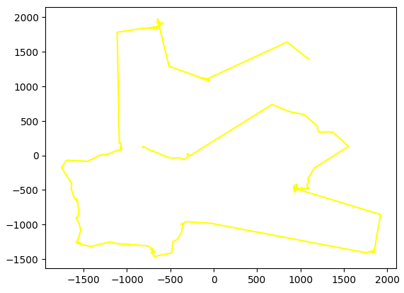
To form the cartesian plots, the rectangular X and Y coordinates were produced by multiplying the distance with cos(theta) and sin(theta). The four individual maps below provide pieces of information that form the entire map of the room.
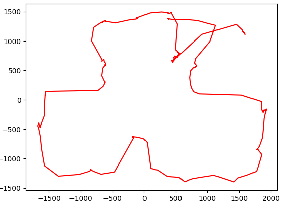
(0,0)ft
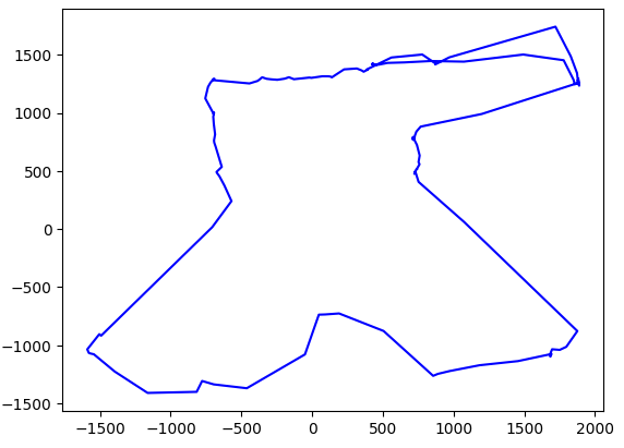
(0,3)ft
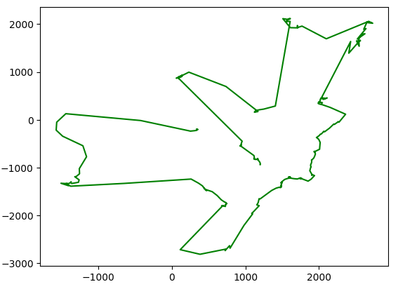
(5,-3)ft
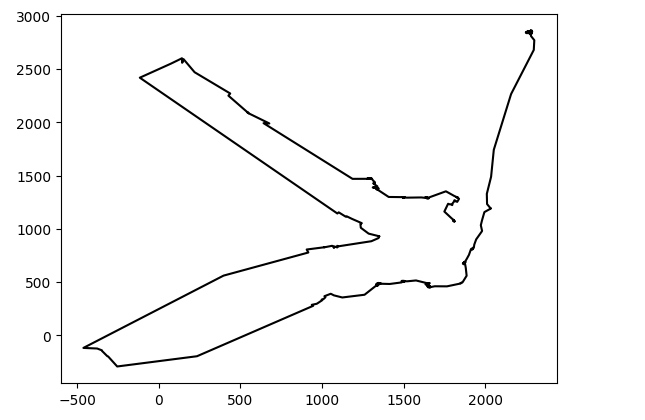
(5,3)ft
(-3,-2)ft
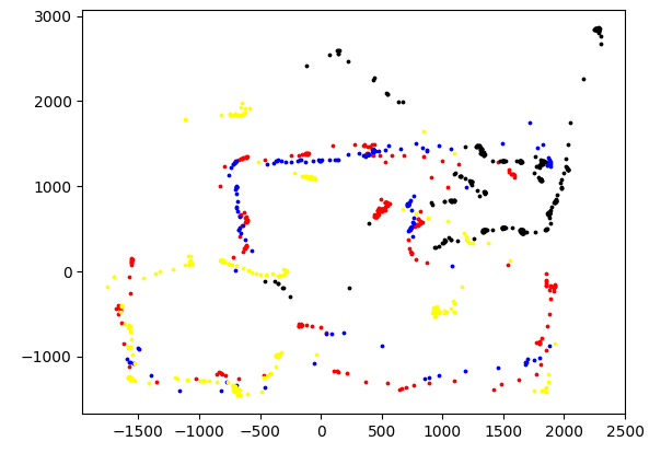
The five separate plots are then merged together to create a final map that resembles the actual room. During merging we used the frame transformations to get each of the plots to the right position. All the calculations for the plots are carried out in millimeter.
Convert to Line-Based Map
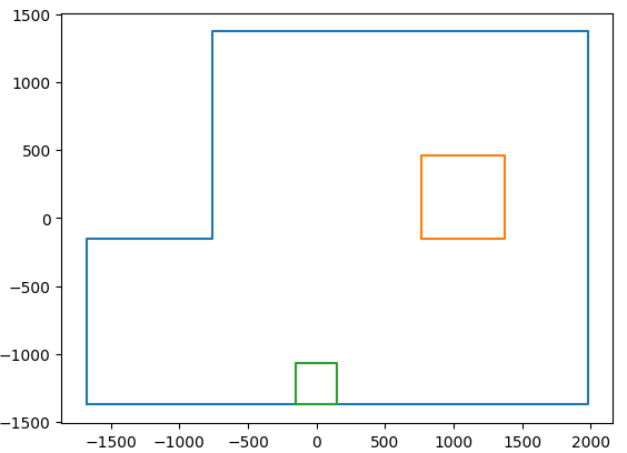
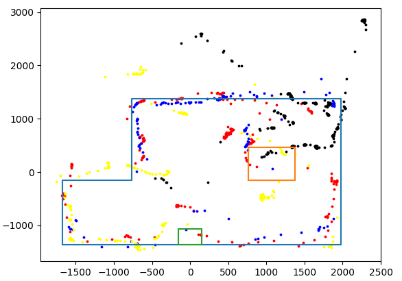
The merged scatter plot displays the outline of the room, but cannot be used in the simulator. To create a line-based map that can be used in the simulator, the dimensions of the room are plotted and overlayed with the merged plot.
x_dim = np.array([-5.5,6.5,6.5,-2.5,-2.5,-5.5, -5.5])
y_dim = np.array([-4.5,-4.5,4.5,4.5,-0.5,-0.5, -4.5])
x_bigbox_dim = np.array([2.5,4.5,4.5,2.5,2.5])
y_bigbox_dim = np.array([-0.5,-0.5,1.5,1.5,-0.5])
x_small_box_dim = np.array([-0.5,0.5,0.5,-0.5,-0.5])
y_small_box_dim = np.array([-4.5,-4.5,-3.5,-3.5,-4.5])

x_dim = x_dim * 304.8
y_dim = y_dim * 304.8
x_bigbox_dim = x_bigbox_dim * 304.8
y_bigbox_dim = y_bigbox_dim * 304.8
x_small_box_dim = x_small_box_dim * 304.8
y_small_box_dim = y_small_box_dim * 304.8

plt.plot(x_dim, y_dim)
plt.plot(x_bigbox_dim, y_bigbox_dim)
plt.plot(x_small_box_dim, y_small_box_dim)
plt.show()
IV. Conclusion
The objective of this lab, to build a virtual map of the static room is successfully satisfied. There were several issues faced during the lab such as robot issues (jerky turning, friction), software and bluetooth related issues. Too much time was spent on the PID and reading the distances, which did not leave enough time to complete the remainder of the tasks. However, this lab was very helpful in understanding the mapping process in robotics. Knowledge gained from this lab with respect to mapping will assist in the future labs. staff was very helpful during the lab and provided important assistance to debug issues.
Collaborators
Askari
