Author: Rahul Goel (NetID: rg764)
I. Objective
The primary objective Lab 7 is to implement a Kalman Filter with the PID scheme designed in Lab 5. The purpose of employing a Kalman Filter is to accomplish the behavior displayed in Lab 5 at a faster pace. This speed up will assist in completing stunts in the next lab (Lab 8).
II. Materials/Software
- 1x SparkFun RedBoard Artemis Nano
- 1x USB A to C Cable
- 1x Fully Assembled Robot (Artemis, Batteries, TOF Sensors, IMU)
- Measuring Tape
- Obstacle for the Robot (Wall)
III. Procedure/Design/Results
Prelab
Lectures- Implementing a Kalman Filter (see references for links) are reviewed prior to initiating the lab work.
Step Response
A step response is carried out by driving the car against a wall while recording motor input values and ToF sensor output. The chosen PWM value (80) corresponds to what I used in Lab 6. The program is configured so that the PWM value is clipped at 80. To implement a step response, I issued a ping from Jupyter, which then triggered the step response in Arduino. I used a counter to get the PWM step for the motors. The step response graphs (distance vs time and PWM vs time) are shown below.
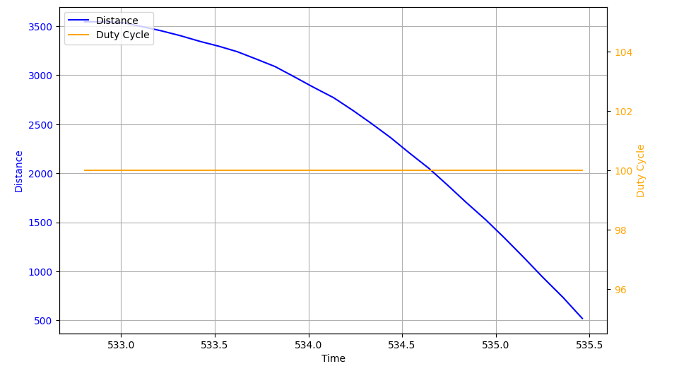
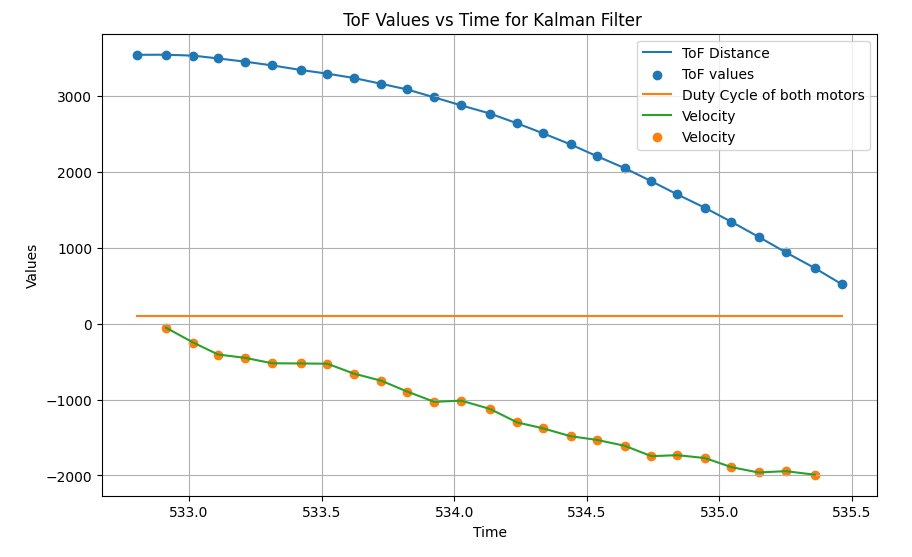
The measured steady state speed is calculated to be 510 mm/s and the 90% rise time is around 2.0 seconds. The A and B matrices are calculated in the following steps.
Kalman Filter Setup
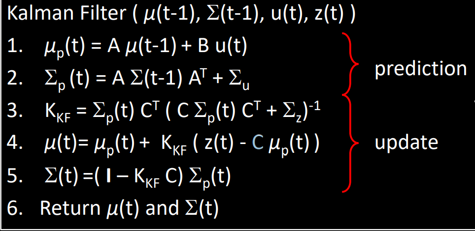
A Kalman Filter predicts the robot’s position using the state space model and then updates that forecast based on sensor measurements. This function is demonstrated below:
In order to determine the A, B, and C matrices, a state space model was developed for the robot. For our robot, we used the distance to the wall (our position), and the robot’s velocity. This is shown in the model below:
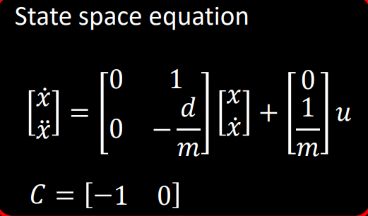
The d and m matrices are calculated as per the code snippet below.
velocity  = 510 mm/s
rise time = 2.0 s
d = 1/velocity
d = 1/510
m = -d*(rise time)/ln(0.1) = 0.0017
-d/m = -1.15
1/m = 588
delta_t = 1 / sampling_rate
sampling_rate = 79
delta_t = 0.0127
Based on the calculated d, m, and delta_t values above, the A and B matrcies are calculated as per below.
A = np.array([[0, 1], [0, -1.15]])
B = np.array([[0], [588]])
C = np.array([[-1, 0]])
Delta_T = 0.0127
A_d = np.identity(2) + Delta_T * A
B_d = Delta_T * B
A_d = [[1.       0.0127  ]
[0.       0.985395]]

B_d = [[0.    ]
[7.4676]]
Sanity Check - Kalman Filter
Once the A, B, and C matrices are identified, the Kalman filter algorithm is implemented on Jupyter (Python) to sanity check the calculations.
def kf(mu,sigma,u,y):
    mu_p = A_d.dot(mu) + B_d.dot(u)
    sigma_p = A_d.dot(sigma.dot(A_d.transpose())) + sig_u
    sigma_m = C.dot(sigma_p.dot(C.transpose())) + sig_z
    kkf_gain = sigma_p.dot(C.transpose().dot(np.linalg.inv(sigma_m)))
    y_m = y-C.dot(mu_p)
    mu = mu_p + kkf_gain.dot(y_m)
    sigma=(np.eye(2)-kkf_gain.dot(C)).dot(sigma_p)

    return mu,sigma
To assess the various outcomes, several sigma_1, sigma_2 values were tested. Higher values for sigma_1 and sigma_2 indicate that the model is unclear and that the sensor values are used. Higher sigma_3 values indicate that there is a lot of sensor noise, hence more trust is placed in the model.
Sigma_1 = 50, Sigma_2 = 50, Sigma_3 = 5
Sigma_1 = 5, Sigma_2 = 5, Sigma_3 = 50
IV. Conclusion
There were several issues faced during the lab such as hardware faults, software bugs (BLE and hardfaults). Overcoming these challenges was very satisfying and the knowledge gained from this lab in regards to implementing the Kalman Filter will be very useful in the future labs. The Lab 7 guideline as well as the staff was also extremely helpful during the lab.
