Author: Rahul Goel (NetID: rg764@cornell.edu)
I. Objective
The primary objective of this lab is to perform localization on the real robot, using only the update step of the Bayes Filter. Localization is the process of determining where a robot is located with respect to its environment.
II. Materials/Software
- Fully Assembled Robot (Artemis, ToF Sensors, IMU, Motor Drivers)
- Jupyter Lab
III. Procedure/Design/Results
Setup
Lab 11 Bayes filter implementation and the provided optimized Bayes filter implementation are utilized to perform localization on the virtual robot. Once the localization on the virtual robot is successful, the real robot undergoes localization. For this lab, the robot is placed in the following 4 marked positions on the map to attain sensor readings:
- (-3 ft ,-2 ft ,0 deg)
- (0 ft ,3 ft ,0 deg)
- (5 ft ,-3 ft ,0 deg)
- (5 ft ,3 ft ,0 deg)
At the abovementioned locations, the Tof sensors shall take 18 sensor readings at 20 degree increments starting from 0 degrees to 340 degrees (0, 20, 40, …, 340). These readings shall be passed into the RealRobot class module in Python where the 18 sensor readings are stored and utilized in the update step to determine the robot’s belief level and current position.
Test Localization in Simulation
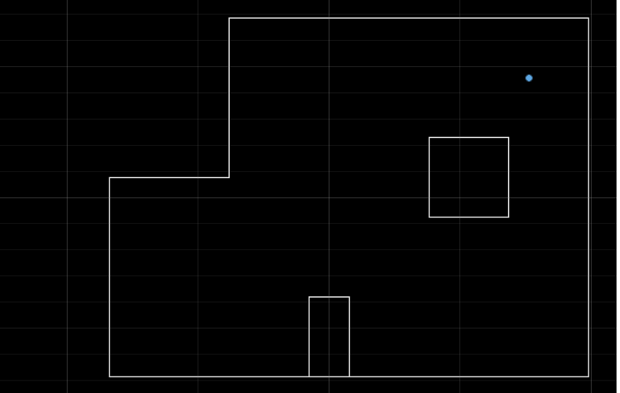
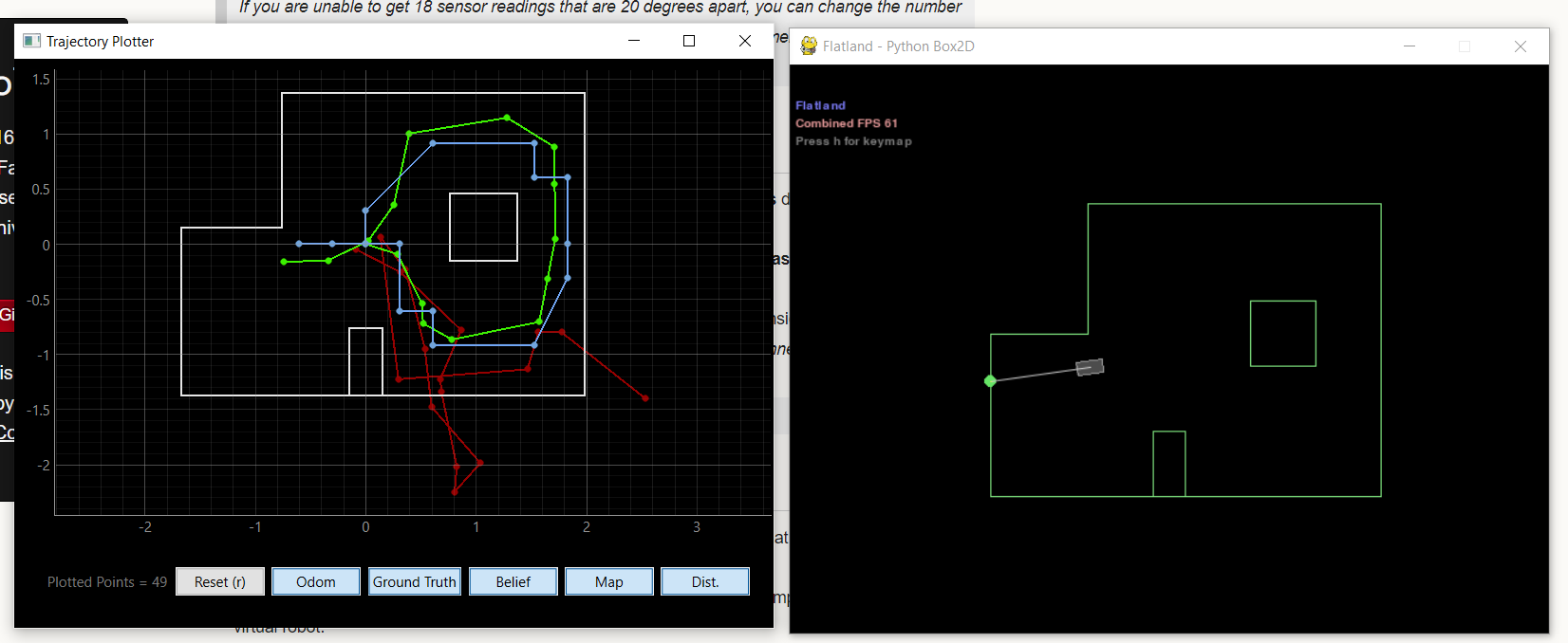
The provided localization implementation is first tested to confirm capability, before proceeding to the real robot. As seen in the plot below, the ground truth (blue), and the robot belief (green) are very similar indicating that the software demonstrates accurate implementation.
Update Step on Real Robot
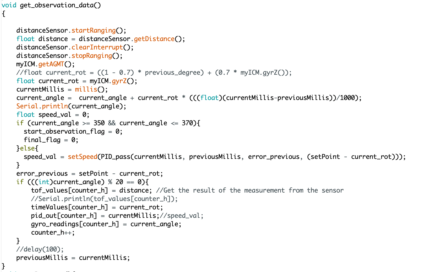
The task involves updating the robot's localization on a map using Time-of-Flight (ToF) sensor readings. This update step entails implementing Proportional-Integral-Derivative (PID) control with the gyroscope, enabling the robot to take 18 sensor readings at 20-degree intervals, covering a full 360-degree rotation (0, 20, 40, ..., 340 degrees). The process involves smoothly rotating the robot while integrating gyroscope values to capture distance readings at each 20-degree increment.
To integrate gyroscope values, the current rotation rate (in radians/second) is multiplied by the time interval between the current and previous readings, and the resulting values are summed over all rotations. These sensor readings, along with the associated rotation values, are stored in an array and then passed into a Python module called RealRobot class to determine the robot's belief location.
A notable adjustment in the code is programming the robot to halt if the current angle falls within the range of 350 to 370 degrees. This ensures that the robot stops even if it doesn't complete a precisely 360-degree turn.
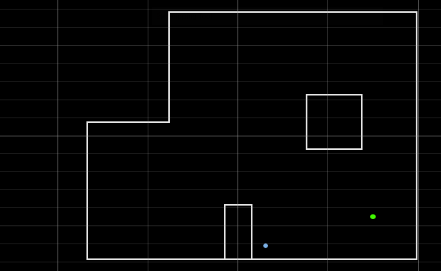
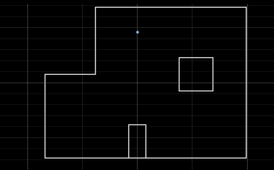
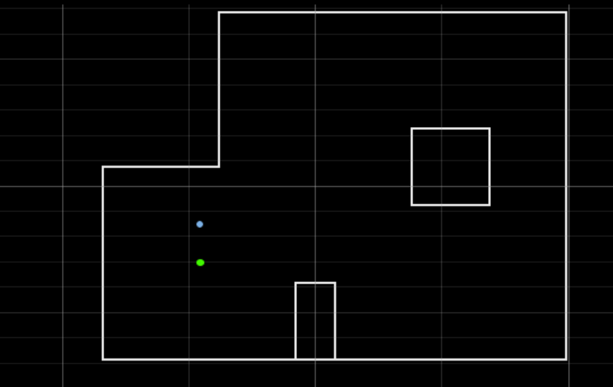
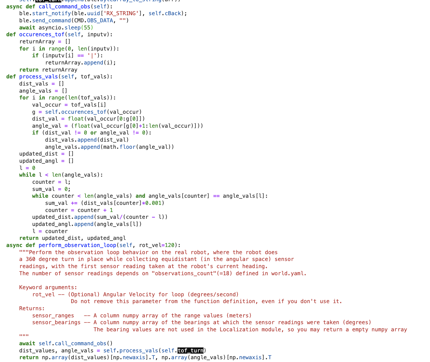
Once the robot is able to capture and transmit readings adequately, Jupyter Lab framework is setup to receive the readings, parse the data (ToF values, angle values), and feed the ToF readings to the perform_observation_loop function. As seen in the image below, there was a need to process and omit some reoccurring data. This was so as the robot would send multiple ToF readings for each 20 degrees increment. The processing omits multiple sensor readings at the same degree increment. Once the data is processed, it is send to the perform_observation_loop function as a np array. The program calculated the new belief position and probability for the four points on the map which is displayed in the images below.
Results
(5,3)
Ground truth pose: (1.524, 0.914, 0.000)
Computed belief pose: (1.524, 0.914, 10.000)
Resultant error: (0.000, 0.000. -10.000)
This result is quite interesting for a few reasons. Firstly, although the robot’s position seems spot-on, there’s a slight ten-degree difference in its orientation. This could be due to either a small error in how the robot’s observation control loop operates or a slight misjudgment in its initial orientation.
Additionally, the confidence level in this position is maxed out at 1.0, indicating complete certainty in its accuracy. This level of confidence was somewhat surprising because typically, even minor variations in sensor readings would suggest alternative possible positions on the grid.
(5,-3)
Ground truth pose: (1.524, -0.914, 0.000)
Computed belief pose: (0.305, -1.219, 110.000)
Resultant error: (1.219, 0.305. -110.000)
This result is less promising that the first. Both localizations at this position resulted in the same estimated position, 4 feet in the x direction, and 1 foot in the y direction, offset. It is also well over a right turn off on orientation. I expect this is due to the nature of that corner of the arena to look very similar to a rotating low-resolution TOF sensor from a number of positons.
(0,3)
Ground truth pose: (0.000, 0.914, 0.000)
Computed belief pose: (0.000, 0.914, -180.000)
Resultant error: (0.000, 0.000, 180.000)
(-3,-2)
Ground truth pose: (-0.914, -0.914, 0.000)
Computed belief pose: (-0.914, -0.405, 180.000)
Resultant error: (0.000, -0.509, -180.000)
IV. Conclusion
I don’t think these localization results necessarily prove that some poses localize better than others. Each location had variations in pose across runs, even if it was just in orientation. I believe a significant portion of the uncertainty stems from the low resolution of the observations. Relying on a single, potentially noisy data point to extrapolate the distance to the nearest obstacle across a whole 20-degree range might not fully leverage the capabilities of the robot.
Moreover, considering the jerky nature of the robot’s rotation in place, I’m not entirely confident that the readings were as precisely separated as the localization assumes. If I were to repeat this experiment, I’d take more than 18 readings and adjust the localization code to account for the true reading bearings, aiming for better results across all positions.
